Layout View
The Layout view is the primary workspace. It shows how every slit, in every diffraction order, maps onto the detector focal plane — updated in real time as you change parameters.
Table of contents
- Central Plot
- Mode Summary Card
- Quick Action Chips
- Grating Rotation Section
- Computed Line Segments
- Spectra Plot
- Drag-n-Drop Support
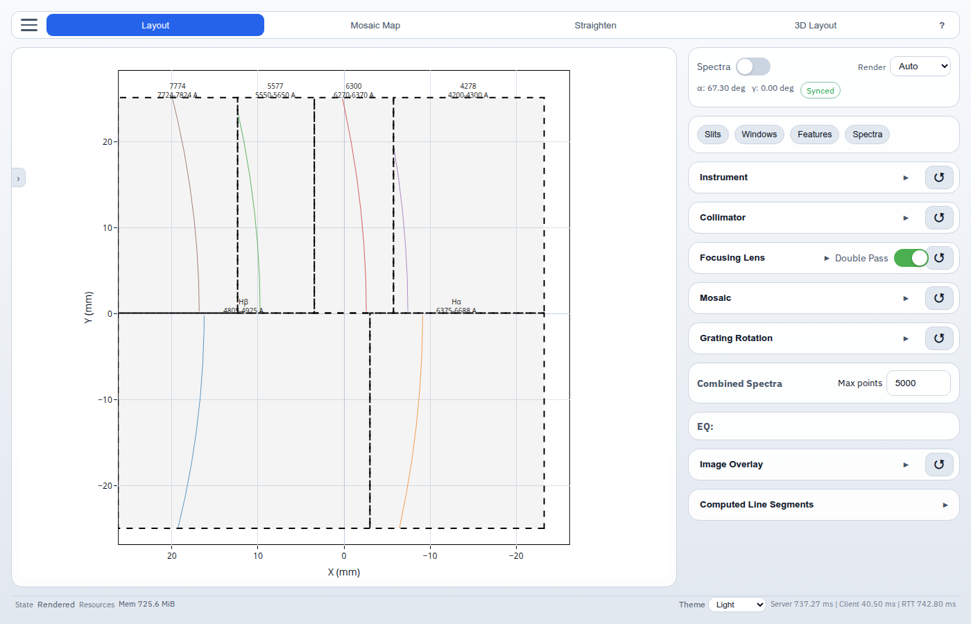
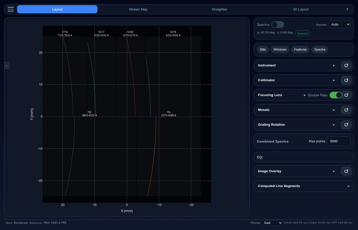
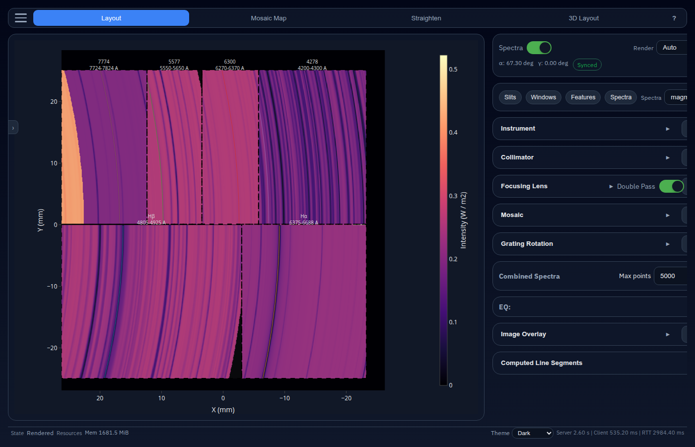
Central Plot
The large Plotly chart in the center of the screen is the focal-plane map. Each colored line segment represents a range of wavelengths from one slit in one diffraction order.
Layer Controls
A collapsible panel sits in the top-left corner of the plot. Use it to show or hide individual rendering layers:
| Layer | Description |
|---|---|
| Heatmap | 2-D intensity map of solar spectrum |
| Lines | Spectral line segments for each slit × order |
| Image | Reference image loaded via Image Overlay |
| Annotations | Wavelength labels from the Spectral Features editor |
Each layer has an opacity slider for blending.
Color Scale
- Linear / Log toggle — switch between linear and logarithmic intensity scaling.
- Auto button — snap the color range to the data minimum and maximum.
- Dual-range slider — manually set the minimum and maximum of the color scale.
Plot interaction
| Action | Effect |
|---|---|
| Click + drag | Pan |
| Scroll | Zoom |
| Double-click | Reset view |
| Hover | Tooltip with wavelength, intensity, and pixel position |
Mode Summary Card
Always visible at the top of the sidebar.
| Control | Description |
|---|---|
| Spectra toggle | Switch between geometry-only and spectra-mapped colour mode |
| Render policy | Auto (live) or Manual (explicit render button) |
| α / γ display | Current grating rotation angles |
| Dirty badge | Synced or Unsaved changes — click to force re-render |
Quick Action Chips
Below the mode summary, four buttons open floating editor windows:
- Slits — define the physical slit positions and sizes.
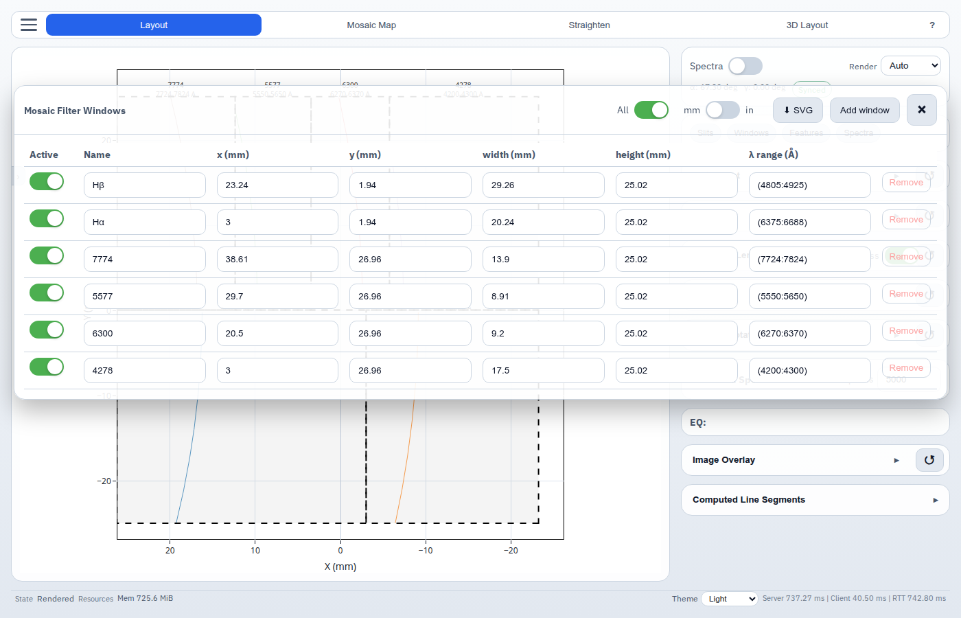
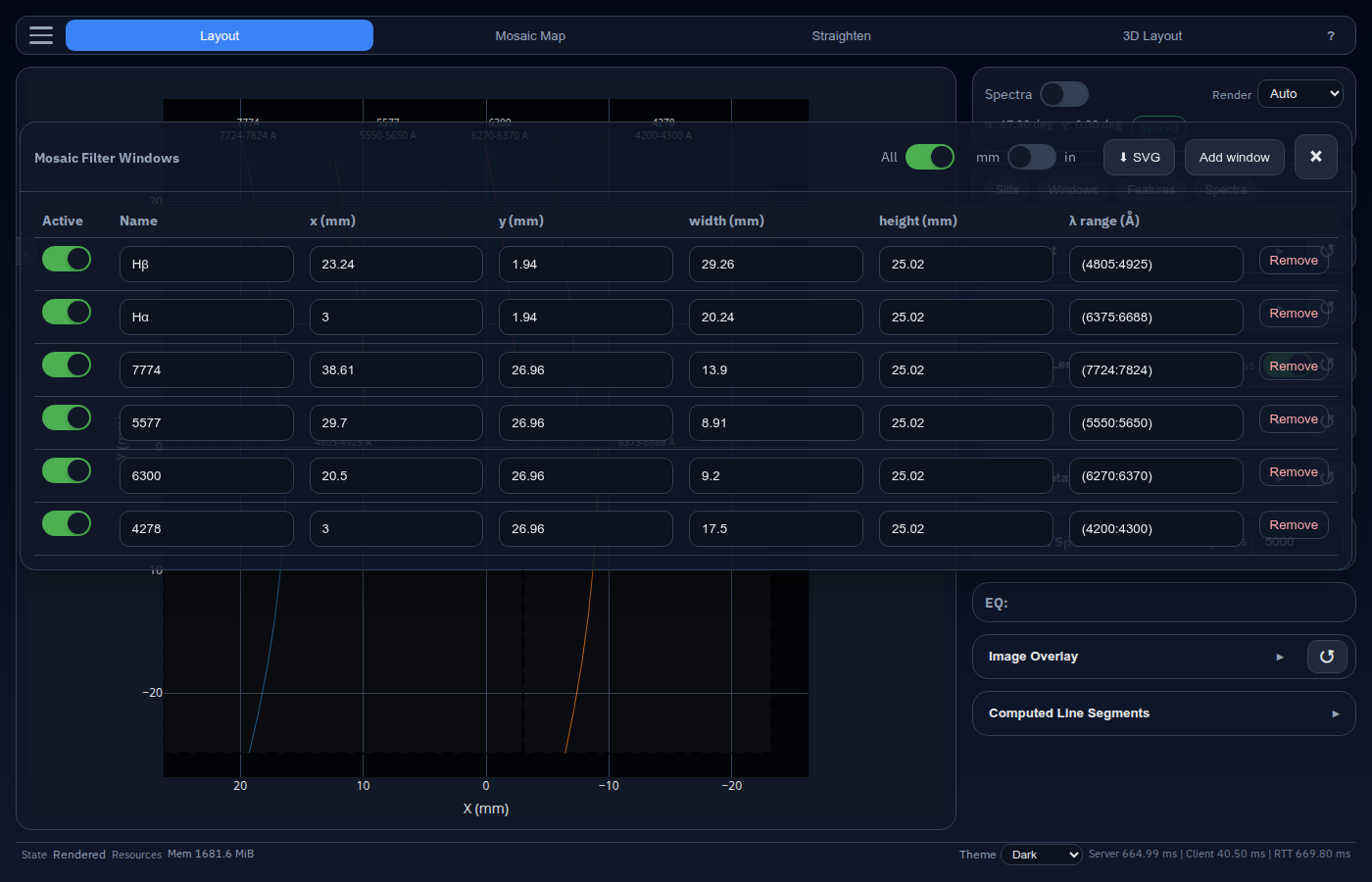
- Windows — define the detector mosaic windows.
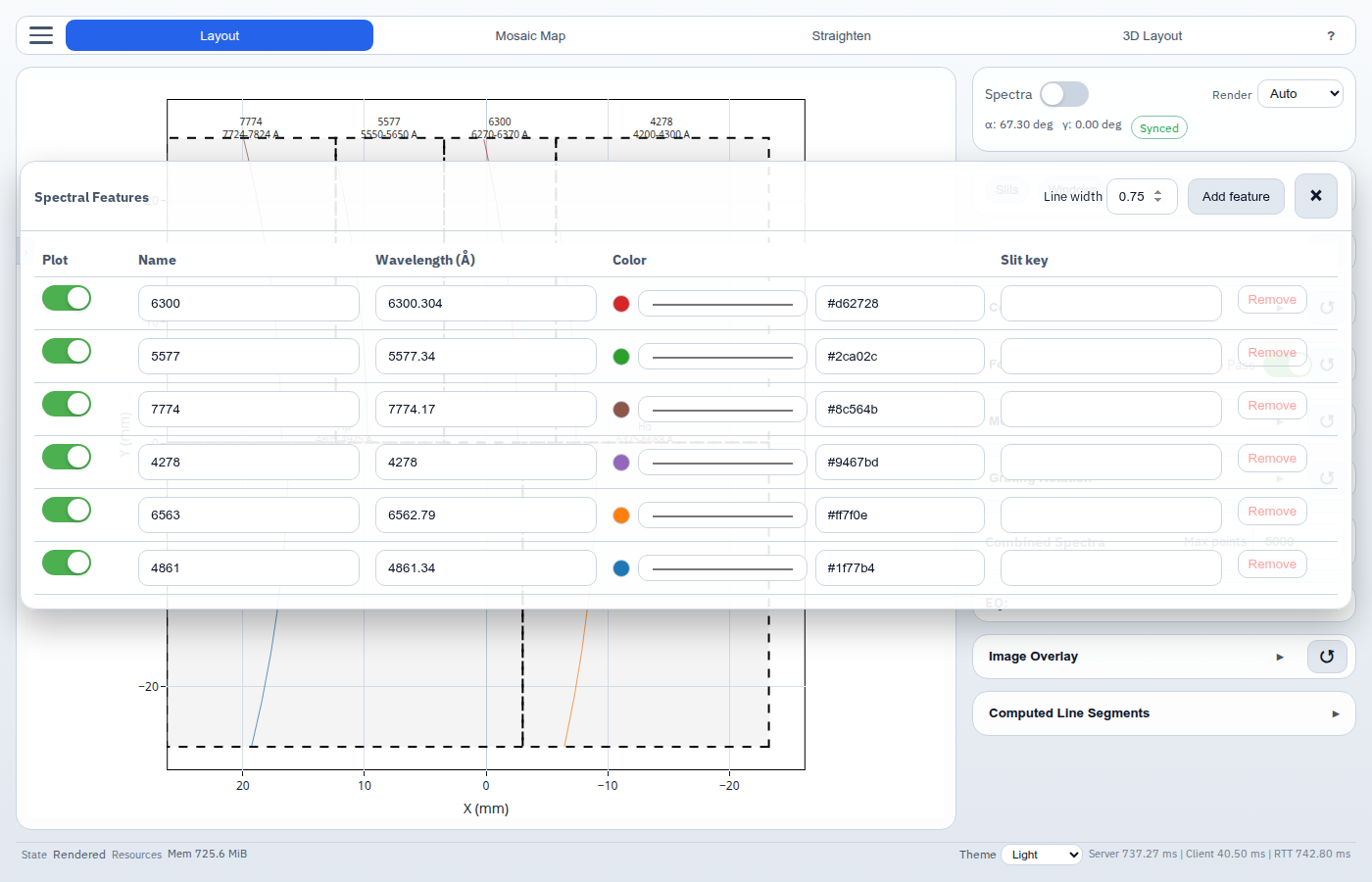
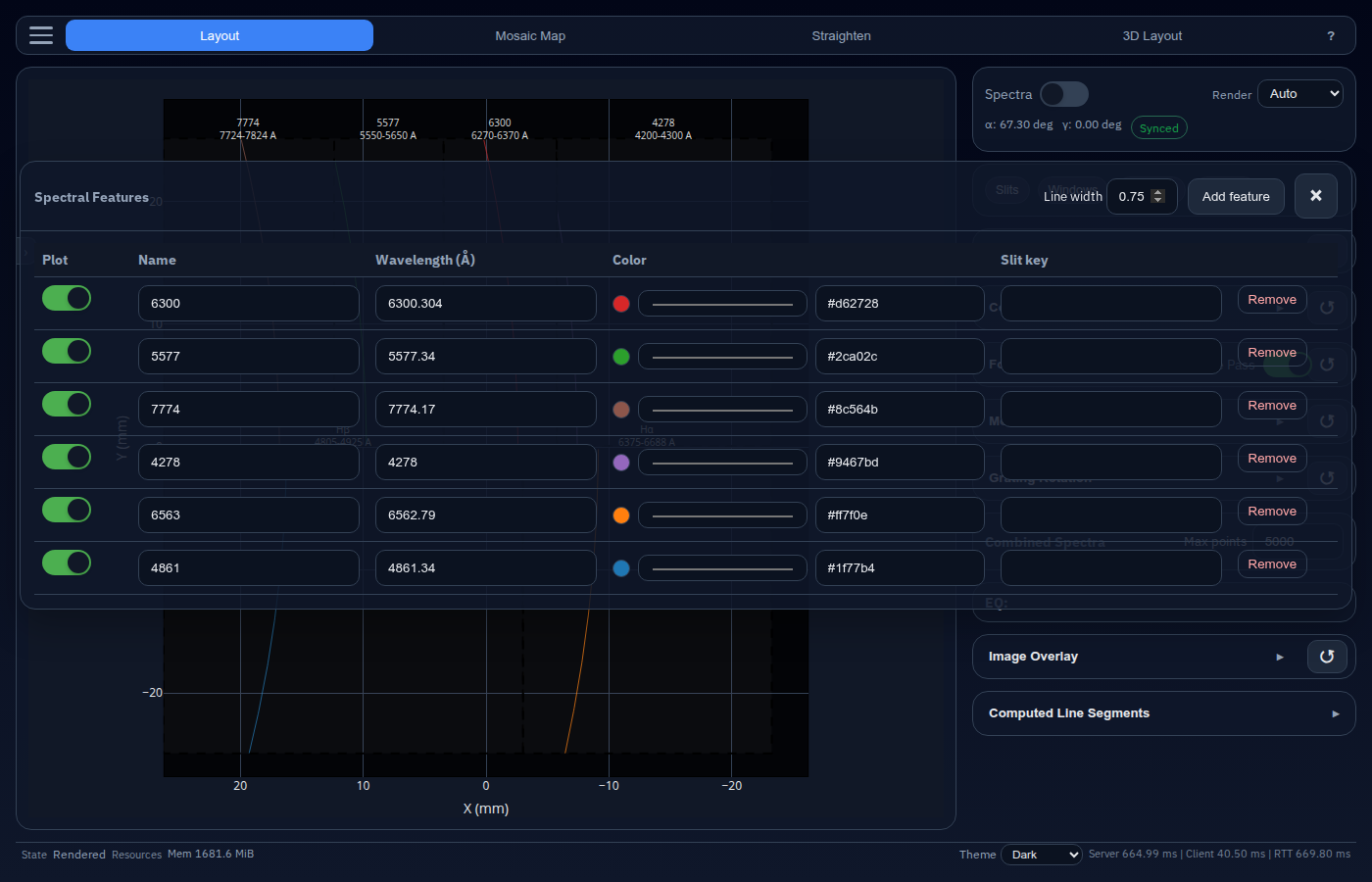
- Features — annotate spectral emission/absorption lines.
- Spectra - select which components are mixed, and to what ratio, for the spectrum run through the instrument.
- Spectra Colormap — (visible in spectra mode) choose the colormap for mapped spectra.
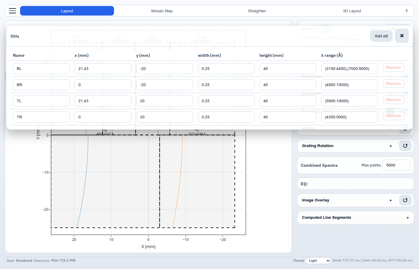
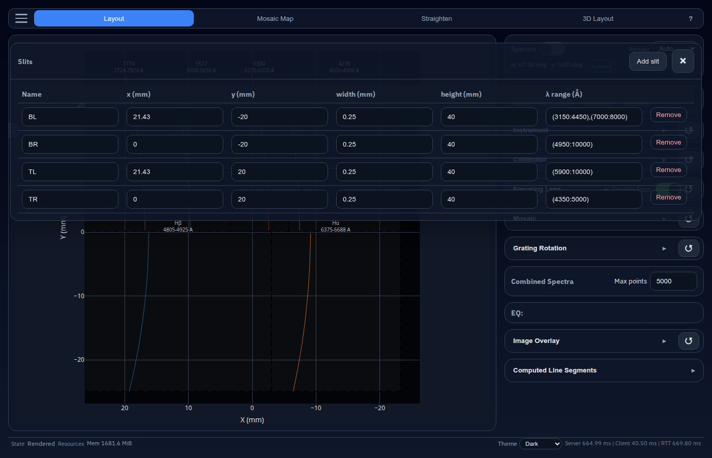
Slits
This control window allows adding and removing entrance slits.
Windows
This control window adds or removes filter panels from the focal plane “mosaic”.
Features
This control window adds or removes/disables spectral features shown in the line plots.
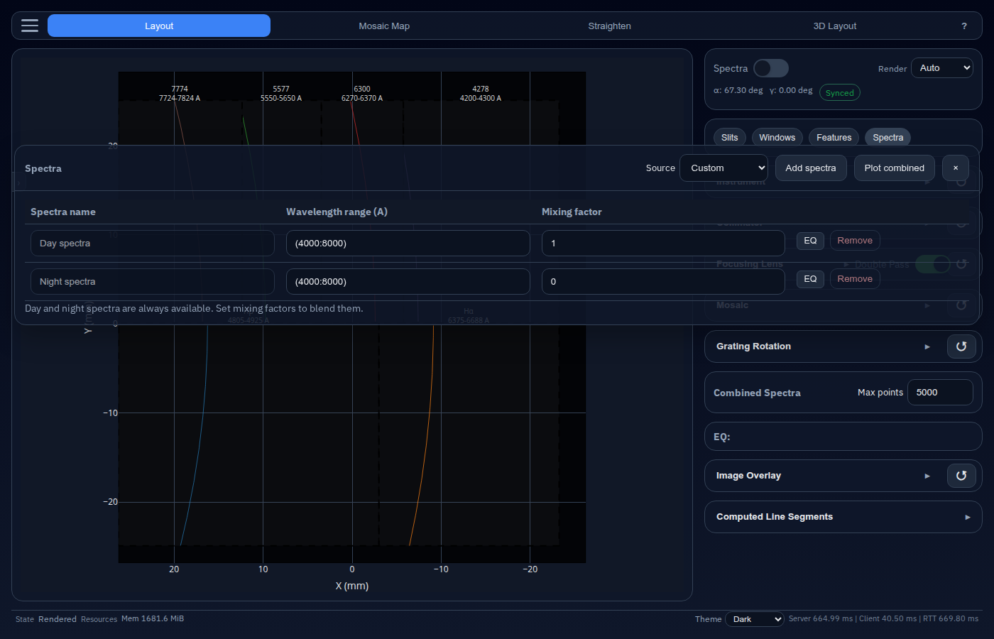
Spectra
This control window adds or removes/disables different spectra (wavelength vs. intensity), and mixes them together:
\[I(\lambda) = \sum_n s_n I_n(\lambda)\]
Spectra EQ
Each spectra row has an EQ button that opens the per-spectrum equaliser. The EQ editor lets you shape a piecewise-linear gain curve $G(\lambda) \in [0, 1]$ that multiplies the raw irradiance before mixing:
\[I_\text{eff}(\lambda) = \sum_n s_n \, G_n(\lambda) \, I_n(\lambda)\]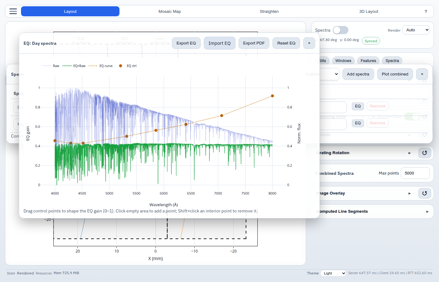
The chart shows three overlaid traces:
| Trace | Axis | Description |
|---|---|---|
| Raw | Right (norm. flux) | Original normalised irradiance of the spectrum |
| EQ×Raw | Right (norm. flux) | Irradiance after EQ gain is applied |
| EQ curve | Left (EQ gain) | Piecewise-linear gain function |
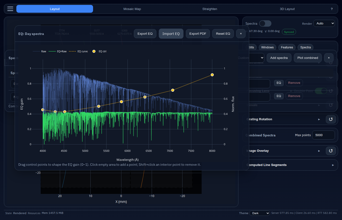
Control-point interactions:
| Gesture | Effect |
|---|---|
| Click empty area | Add a new control point at that position |
| Drag a point | Move the point (boundary points are gain-only; interior points move freely) |
| Shift+click interior point | Remove the point |
The header toolbar provides additional actions:
| Button | Description |
|---|---|
| Export EQ | Download the current control points as a JSON file |
| Import EQ | Load previously exported control points from a JSON file |
| Export PDF | Save the EQ chart as a PDF |
| Reset EQ | Remove all custom points and revert to flat gain = 1 |
Grating Rotation Section
The most frequently used section. Controls the two grating orientation angles and numerical resolution.
| Control | Range | Description |
|---|---|---|
| α offset | 0 – 90° | In-plane grating tilt (sometimes called the blaze angle offset). Drag the slider or type a value. |
| γ offset | −30 – +30° | Out-of-plane grating rotation (conical diffraction angle). |
| Angular grid samples | 51 – 801 | Number of discrete angular positions computed per segment. Higher values are slower. |
| Angular step | 0.001 – 10° | Step size used when sweeping angle during segment tracing. |
| Finer / Coarser | — | Halve or double the angular step with one click. |
The backend internally uses −α. The UI displays the positive convention; the sign flip is applied automatically.
Computed Line Segments
A read-only table at the bottom of the sidebar lists every segment that was calculated in the last render: slit name, diffraction order, wavelength range, and pixel coordinates. It is hidden when the layout has not yet been rendered.
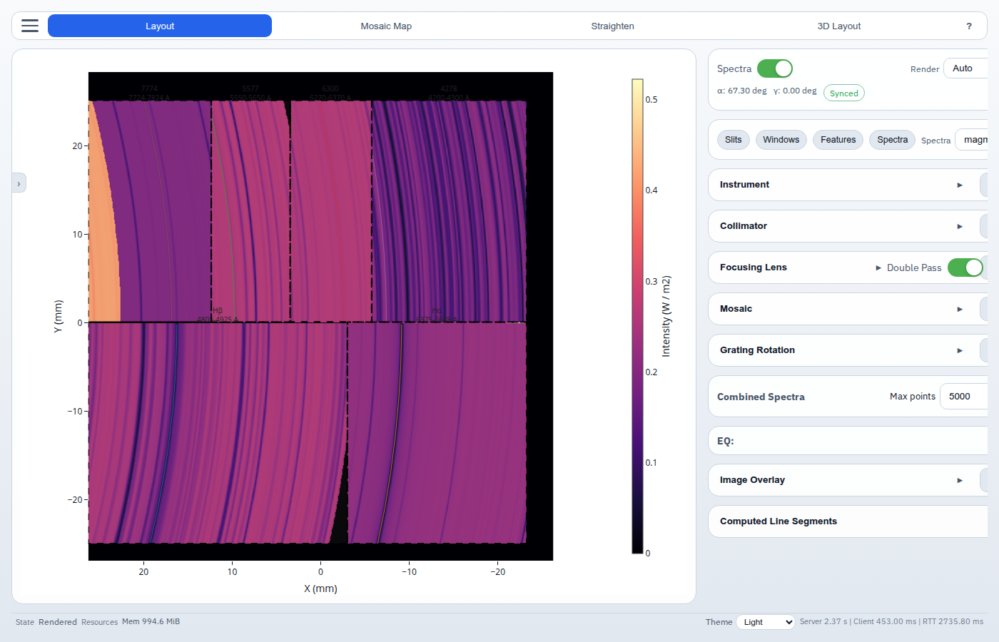
Spectra Plot
If a spectral window is specified with some wavelength range, enabling “Spectra” will simulate the solar spectra on the focal plane of the instrument. The solar spectra image is rendered below the mosaic windows in layout view.
Drag-n-Drop Support
The layout view supports drag-n-drop for loading instrument TOML files and reference images. Try dragging a file from your computer onto the layout view to load it!